A quick way to compare two lists in your spreadsheet is to use Excel’s unique highlight feature. This feature highlights the items in a list that are not found in the other list. This way you know exactly what items are missing from your lists.
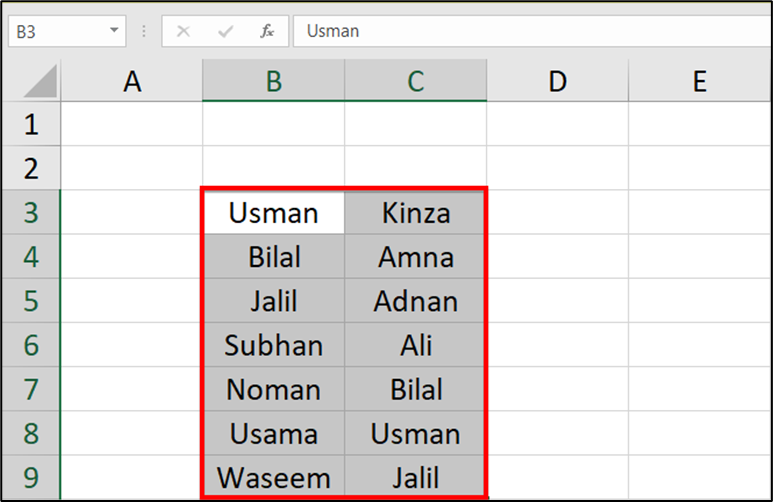
Step 1- First, select the lists you want to compare in your spreadsheet.
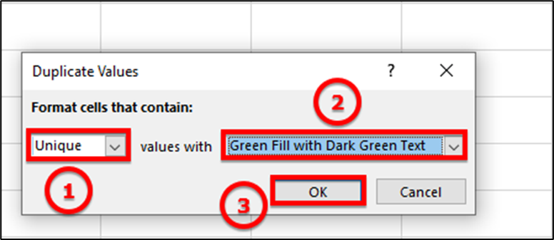
Step 3- On the “Home” tab, in the “Styles” section, click Conditional Formatting > Highlight Cells Rules > Duplicate Values.
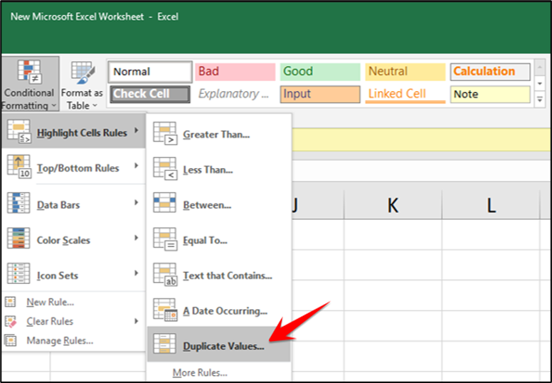
Then apply your changes to your lists by clicking “OK.”
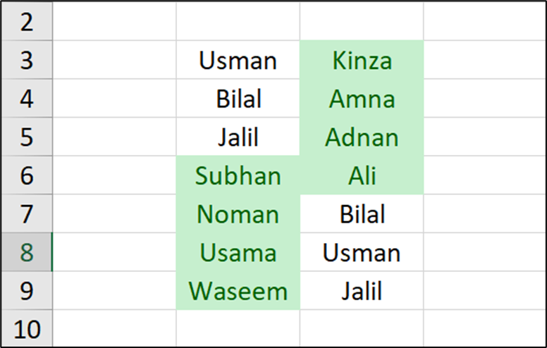
Excel will highlight the missing items in your lists. For example, in your first list, you will have those items highlighted that are missing from the second list, and so on.