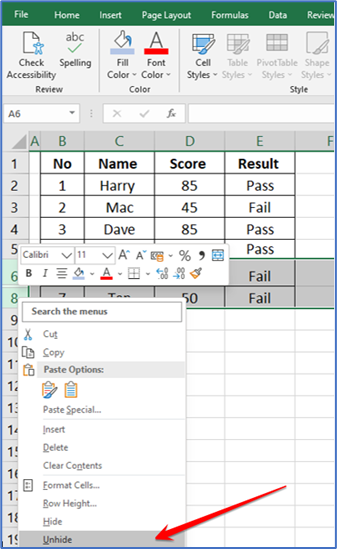
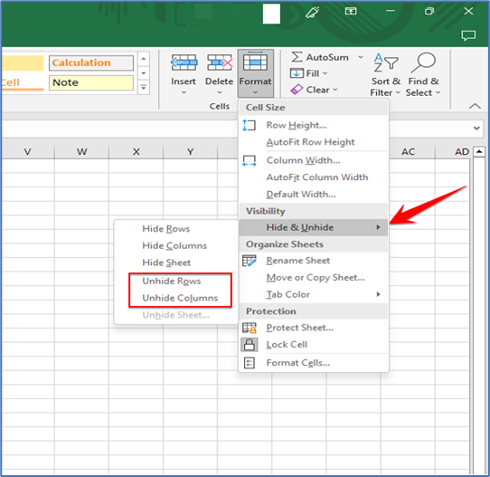
Alternately, select the Format > Hide & Unhide > Unhide Rows option from Excel’s “Home” tab in the ribbon. This also applies to
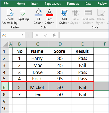
You are ready to go.
How to Unhide Specific Rows in Excel
Use the following technique to make only certain rows visible while keeping all other hidden items hidden.
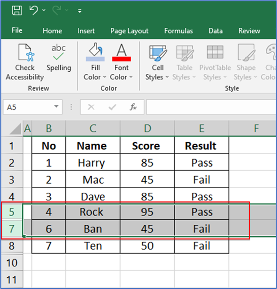
Click the header of the row above the one you want to make visible by hiding it. For instance, click the header for row 5 to make row 6 visible
Now, press and hold down the Shift key on your keyboard and click the header of the row that’s beneath your hidden row. In the above example, you’ll click the header for row 7 (while the Shift key is held down).
Note that you select all the rows between your clicked items when you click a row header while holding down Shift. This also selects the hidden content that you will later choose to reveal.